【Python自前実装】直線フィッティング

線形回帰を自前実装

クラスの仕様は大体sklearnに合わせています。
ポイントはxに1の列を加えているところです。

# 線形回帰クラス
class LinearRegression:
    
    def __init__(self):
        pass

    def fit(self, x, t):
        X = self._add_ones(x)
        self.w = np.linalg.inv(X.T @ X) @ X.T @ t
        
    def predict(self, x):
        X = self._add_ones(x)
        return X @ self.w

    def score(self, x, t):        
        t_pred = self.predict(x)
        t_mean = t.mean()
        return 1 - np.sum((t - t_pred) ** 2) / np.sum((t - t_mean) ** 2)

    def _add_ones(self, x):
        ones = np.ones((x.shape[0], 1))
        return np.hstack((ones, x))

ソース

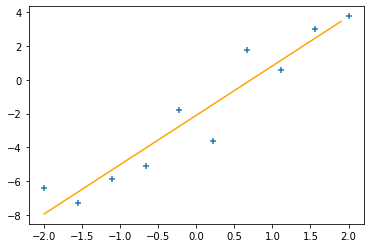
sklearnを使った時とほぼ同じ結果が得られました。

import matplotlib.pyplot as plt
import numpy as np

# 線形回帰クラス
class LinearRegression:
    
    def __init__(self):
        pass

    def fit(self, x, t):
        X = self._add_ones(x)
        self.w = np.linalg.inv(X.T @ X) @ X.T @ t
        
    def predict(self, x):
        X = self._add_ones(x)
        return X @ self.w

    def score(self, x, t):        
        t_pred = self.predict(x)
        t_mean = t.mean()
        return 1 - np.sum((t - t_pred) ** 2) / np.sum((t - t_mean) ** 2)

    def _add_ones(self, x):
        ones = np.ones((x.shape[0], 1))
        return np.hstack((ones, x))

# データの数
N = 10

# 乱数を固定
np.random.seed(1)

# バラつきのある y = 3x - 2 のデータを作成
x = np.linspace(0, 1, N).reshape(-1, 1)     # 0 〜 1 までの乱数を N 個つくる
x = x * 4 - 2                               # 値の範囲を -2 〜 2 に変更

y = 3 * x - 2  # y = 3x - 2
y += np.random.randn(N, 1)  # 標準正規分布（平均 0, 標準偏差 1）の乱数を加える

# 線形回帰のモデルを作成
model = LinearRegression()
# 学習
model.fit(x, y)

# 予測直線表示のためのxを作成 予測するために行列にする(reshape)
x2 = np.arange(-2, 2, 0.1).reshape(-1,1)
y2 = model.predict(x2)

# 係数、切片、決定係数を表示
print('係数', model.w[1:])
print('切片', model.w[0])
print('決定係数', model.score(x, y))

# グラフ表示
plt.scatter(x, y, marker ='+')
plt.plot(x2, y2, color='orange')
plt.show()

偉人の名言

参考文献

パターン認識と機械学習 上巻

動画

なし