【Python自前実装】曲線フィッティング

乱数の固定

現象が再現するように乱数を固定します。

# ランダムシードを設定する(乱数を固定する)
np.random.seed(1)

入力空間と特徴空間

今回のプログラムでは入力空間は1次元です。
その入力空間の元 $x$ を非線形写像 ${\boldsymbol\phi}(x)=(x^0,x^1,\ldots,x^{M-1})^T$ で写した特徴空間で回帰します。
目標値 $t$ と入力値 $x$ の関係は $t=\sin(x)+\epsilon$ で $\epsilon$ は平均が $0$ 、標準偏差が $0.2$ の正規分布に従います。
計画行列 $\boldsymbol\Phi$ は以下の式で表されます。

$\begin{eqnarray} {\boldsymbol\Phi}&=&\begin{pmatrix}{\boldsymbol\phi}(x_1)^\top\\\vdots\\{\boldsymbol\phi}(x_N)^\top\end{pmatrix}\\ &=&\begin{pmatrix} \phi_0(x_1) & \phi_1(x_1) & \cdots & \phi_{M-1}(x_1)\\ \phi_0(x_2) & \phi_1(x_2) & \cdots & \phi_{M-1}(x_2)\\ \vdots & \vdots & \ddots & \vdots\\ \phi_0(x_N) & \phi_1(x_N) & \cdots & \phi_{M-1}(x_N)\\ \end{pmatrix}\\ &=&\begin{pmatrix} x_1^0 & x_1^1 & \cdots & x_1^{M-1}\\ x_2^0 & x_2^1 & \cdots & x_2^{M-1}\\ \vdots & \vdots & \ddots & \vdots\\ x_N^0 & x_N^1 & \cdots & x_N^{M-1}\\ \end{pmatrix}\\ &=&\begin{pmatrix} 1 & x_1 & \cdots & x_1^{M-1}\\ 1 & x_2 & \cdots & x_2^{M-1}\\ \vdots & \vdots & \ddots & \vdots\\ 1 & x_N & \cdots & x_N^{M-1}\tag{1} \end{pmatrix}\\ \end{eqnarray}$

ですが、プログラムでは、以下の図1のようにしています。

図1
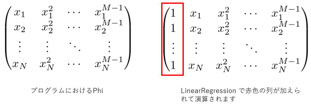
f:id:olj611:20211022181345p:plain:w600

プログラムで最初に作成する Phi は $N\times (M-1)$ であることに注意してください。
sklearn.linear_model.LinearRegression に仕様を合わせているため、計画行列から、成分が1の列を抜いています。
LinearRegression 内で、計画行列は $N\times M$ となります。

# 訓練データxの列ベクトル(入力空間)
x = np.linspace(0, 1, N).reshape(-1, 1)

# 特徴空間作成のためのインスタンスを作成(※成分が1のみの列は作成しないため、M-1を渡す)
dm = DesignMatrix(M-1)

# 入力空間から特徴空間へ写す
# 行列Phi(特徴空間)を作成(※成分が1のみの列は作成していない)
Phi = dm.transform(x)

# 訓練データt=sin(x)の列ベクトルに正規分布に従うノイズを加える
t = true_func(x) + np.random.normal(0, 0.2, N).reshape(-1, 1)

特徴空間で予測する

予測は特徴空間で行います。

# 訓練データt=sin(x)の列ベクトルに正規分布に従うノイズを加える
t = true_func(x) + np.random.normal(0, 0.2, N).reshape(-1, 1)

# 線形回帰のモデルを作成
model = LinearRegression()

# 学習する
model.fit(Phi, t)

コード

import matplotlib.pyplot as plt
import numpy as np

# 計画行列クラス(※成分が1の列は作成しない)
class DesignMatrix:

    def __init__(self, degree):
        self.degree = degree

    def transform(self, x):
        return np.hstack([x**(m+1) for m in range(self.degree)])

# 線形回帰クラス
class LinearRegression:
    
    def __init__(self):
        pass

    def fit(self, x, t):
        X = self._add_ones(x)
        self.w = np.linalg.inv(X.T @ X) @ X.T @ t
        
    def predict(self, x):
        X = self._add_ones(x)
        return X @ self.w

    def score(self, x, t):        
        t_pred = self.predict(x)
        t_mean = t.mean()
        return 1 - np.sum((t - t_pred) ** 2) / np.sum((t - t_mean) ** 2)

    def _add_ones(self, x):
        ones = np.ones((x.shape[0], 1))
        return np.hstack((ones, x))

# 訓練データ作成のための真の関数
def true_func(x):
    return np.sin(2 * np.pi * x)

# ランダムシードを設定する(乱数を固定する)
np.random.seed(1)

# 訓練データ数
N = 10

# 特徴空間の次元(モデルのパラメータ数)
M = 4

# 訓練データxの列ベクトル(入力空間)
x = np.linspace(0, 1, N).reshape(-1, 1)

# 特徴空間作成のためのインスタンスを作成(※成分が1のみの列は作成しないため、M-1を渡す)
dm = DesignMatrix(M-1)

# 入力空間から特徴空間へ写す
# 行列Phi(特徴空間)を作成(※成分が1のみの列は作成していない)
Phi = dm.transform(x)

# 訓練データt=sin(x)の列ベクトルに正規分布に従うノイズを加える
t = true_func(x) + np.random.normal(0, 0.2, N).reshape(-1, 1)

# 線形回帰のモデルを作成
model = LinearRegression()

# 学習する
model.fit(Phi, t)

# 係数、切片、決定係数を表示
print('係数', model.w[1:])
print('切片', model.w[0])

r2 = model.score(Phi, t)
print('決定係数', r2)

# 予測直線表示のためのxを作成 予測するために行列にする(reshape)
x2 = np.linspace(0, 1, 100).reshape(-1,1)

# 行列Phi2(特徴空間)を作成(※成分が1のみの列は作成していない)
Phi2 = dm.transform(x2)

# 予測する
y2 = model.predict(Phi2)

# グラフ表示
plt.scatter(x, t, marker ='+')
plt.plot(x2, y2, color='orange')
plt.show()

f:id:olj611:20210611050620p:plain:w600

偉人の名言

f:id:olj611:20210616172904p:plain:h300
新しいことを勉強してると世の中は怖くありません。
何もしないで、じっとしているから、怖くなるんです。
林家彦六

曲線フィッティング - 最小二乗法
 【Python実装 - sklearn使用】曲線フィッティング

参考文献

パターン認識と機械学習上巻

動画

なし

機械学習基礎理論独習

誤りがあればご指摘いただけると幸いです。数式が整うまで少し時間かかります。リンクフリーです。